


Next: Material and Methods
Up: CALIBRATION OF ELASTIC-PLASTIC MATERIAL
Previous: Elastic Cross-Anisotropic Constitutive Law
Elastic-Plastic Constitutive Law
The most general form of elastic-perfectly plastic incremental stress-strain
relationship can be expressed as [1],
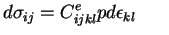 where where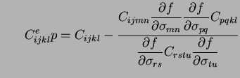 |
(10) |
The coefficient tensor
 is the elastic-plastic tensor of tangent moduli
for an elastic-perfectly plastic material.
The tensor of elastic moduli,
is the elastic-plastic tensor of tangent moduli
for an elastic-perfectly plastic material.
The tensor of elastic moduli,  , can be expressed in terms of
  and
and  as [1],
![$\displaystyle C_{ijkl} = \frac{E}{2(1+\nu)}\left[\frac{2\nu}{(1-\nu)}\delta_{ij}\delta_{kl}+\delta_{ik}\delta_{jl}+\delta_{il}\delta_{jk}\right]$](img34.png) |
(11) |
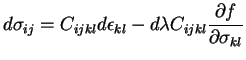
By using Hooke's law and additive decomposition of strain tensors in the elastic and
plastic parts [8] we obtain
 |
(12) |
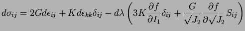
By substituting Eq. (11) into Eq. (12), and with
 it follows
![$\displaystyle d\sigma_{ij}=2Gd\epsilon_{ij}+Kd\epsilon_{kk}\delta_{ij}-d\lambda...
...ma_{mn}}\delta_{mn}\delta_{ij}+2G\frac{\partial f}{\partial \sigma_{ij}}\right]$](img37.png) |
(13) |
Assuming a Drucker-Prager material model, the yield function,  , is
given by,
, is
given by,
 and hence it follows that
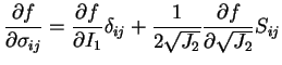 |
(14) |
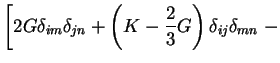
Substituting Eq. (14) into Eq. (13) we have,
 |
(15) |
where  has the form,
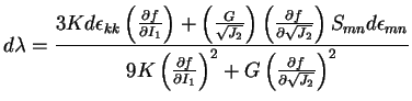 |
(16) |
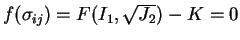
Now, the Drucker-Prager yield condition,f, is given by
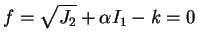 |
(17) |
Combining Eqs. (15), (16) & (17), we have
the most general form of Drucker-Prager elastic-perfectly plastic constitutive
relationship as,
This relationship will be used in assessing one dimensional wave propagation
characteristics of tire shred material described below.
Next: Material and Methods
Up: CALIBRATION OF ELASTIC-PLASTIC MATERIAL
Previous: Elastic Cross-Anisotropic Constitutive Law
Boris Jeremic
2003-11-14
![$\displaystyle \left.
\frac{\left(\frac{G}{\sqrt{J_2}}\right)S_{ij}
+
3K\alpha\d...
...ft(\frac{G}{\sqrt{J_2}}S_{mn}
+
3K\alpha\delta_{mn}\right)\right]d\epsilon_{mn}$](img48.png)